Methodology
Learn more about what geographies are included in the Chicago Community dashboard, how we calculate our estimates, and sources of uncertainty and guidance for using the numbers in your work.
The geographies we cover: community areas, wards, and school board districts
Chicago is divided into 77 community areas, drawn by University of Chicago sociologists in the 1920s. Their boundaries haven't changed since. This gives us a stable baseline that mostly matches how Chicagoans think about neighborhoods, albeit imperfectly.
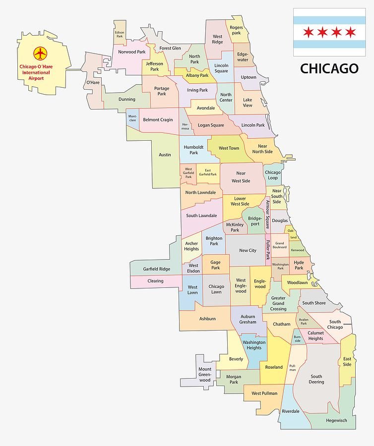
Map of Chicago's 77 community areas.
We also publish profiles for the city's 50 wards, and for its school board districts. Unlike community areas, these are political boundaries, so they are redrawn roughly once a decade to account for population changes.
In order to speak to how an area has changed, rather than how boundaries have changed, we calculate every year of ward and school board district data using the most recent boundaries. For example, Chicago's current ward map took effect in 2023. The 2015 estimate for Ward 1 reflects the 2023 boundaries, not the 2015 boundaries.
How we build these estimates
Most data sources don't publish numbers for community areas, wards, or school board districts directly. We build those numbers from smaller geographies instead, using one of three methods, depending on the source.
1. Most indicators: built from Census tracts
The U.S. Census Bureau publishes results at several levels of geography. We use Census tracts as the building block for our estimates, because they maximize population size while remaining considerably smaller than community areas. A tract is a small area of roughly 4,000 residents. Chicago's 77 community areas are made up of hundreds of them.
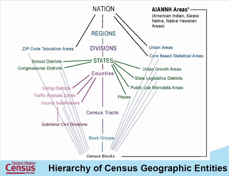
Diagram showing the hierarchy of Census geographic entities. Tracts are the third most granular.
Tract boundaries and community area boundaries, or ward boundaries or school board district boundaries, don't always line up. Most tracts sit inside one community area, but some straddle boundaries. For every indicator, we calculate how much of each tract falls inside a given community area, and weight its data accordingly.
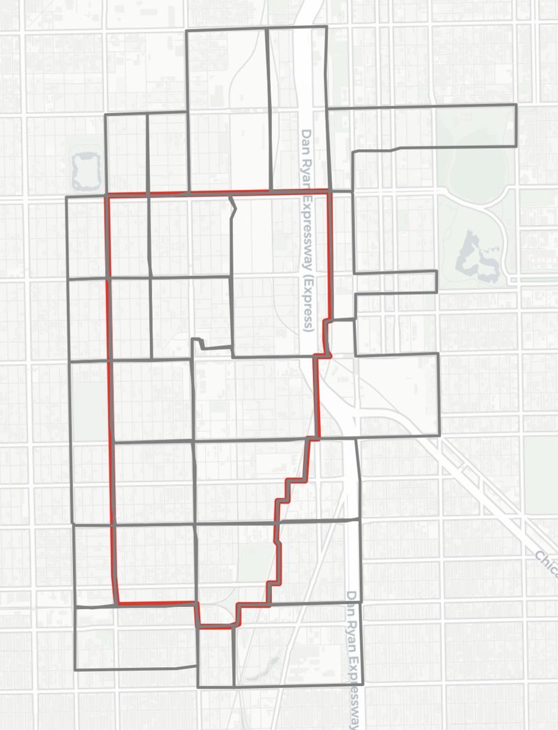
Illustration of Ward 47 (red outline) and the Census tracts that either touch or fall within it (gray outline).
If a tract falls entirely within that red ward boundary, we use the whole tract in our calculation. If a tract just barely touches the border line of the boundary, we end up not using it in our calculation at all. For tracts that don’t cleanly fall in or out of the ward, we use the proportion of the tract that falls within the ward as a weight in our calculation, for example:
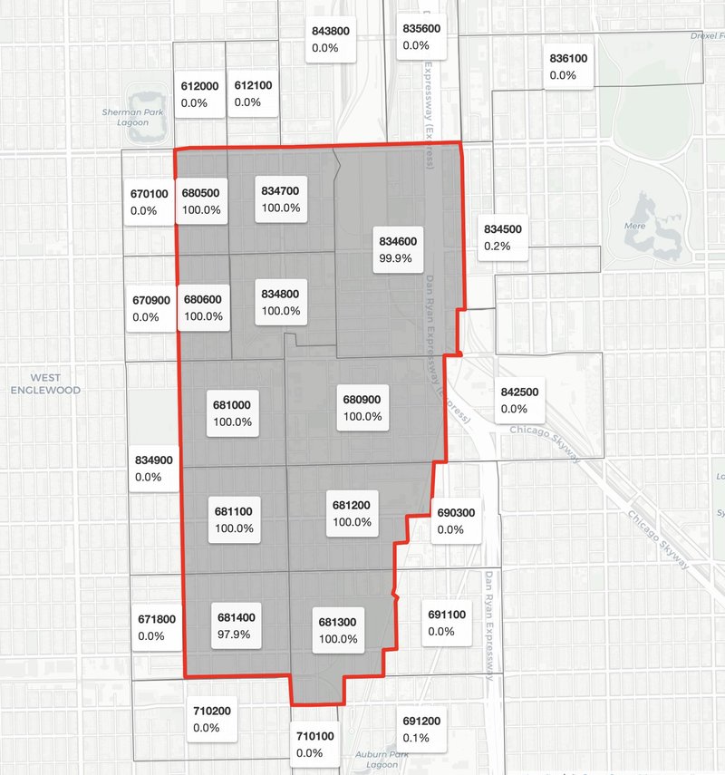
Illustration of Ward 47 (red outline, gray shading) and intersecting Census tracts (light gray) labeled with their name and the proportion of their area that overlaps with the ward.
For example, let’s consider the number of unemployed residents in Ward 47. We sum the count of unemployed residents in each tract directly from the Census. If a tract falls entirely within ward 47, we add its full count to our ongoing sum. If only 1% of a tract falls within ward 47, we count 1% of its unemployed residents. We add this up across every tract that falls within or intersects with Ward 47.
To calculate rates (or proportions), we perform the tract-weighted sum described above for the total population of the table universe, then divide the subgroup population by the total population, e.g., number of unemployed residents / total population in workforce.
Census Reporter helpfully defines table universe as:
[T]he focus of a given data tabulation. For many Census tables, the universe is all people living in the United States and Puerto Rico, but it is not always. For example, the Census Bureau specifically constrains tables about educational attainment, employment, child bearing, and others based on age and other characteristics. Some tables focus specifically on the United States, excluding Puerto Rico, or vice versa. Be sure to take note of the universe when analyzing data and expressing findings about it.
To calculate medians, we perform the tract-weighted sum to estimate the population counts in each bucket we need for our calculation, and then we follow the logic outlined in this Esri blog to derive the median estimate.
2. School-based indicators: built from CPS attendance boundaries
Indicators from Chicago Public Schools work differently. There are two key caveats to consider:
- We calculate estimates for CPS students who live in a community area, not students who attend schools located there. These are often different groups, since kids regularly attend school outside their home neighborhood.
- Our CPS estimates only cover students attending neighborhood schools. In lieu of tracts, we calculate how much of each school's attendance boundary overlaps with each community area, ward, or school board district, and assume that share of students lives there. This necessarily excludes students attending selective enrollment and charter schools, which do not have attendance boundaries. While our statistics exclude students attending choice schools, we think this is a valuable measure of the quality of resources you are entitled to as a resident of each community.
Instead of Census tracts, we use CPS attendance boundaries as our building block geography for school-based indicators. For example, in the below image, we see that 36% of Bass Elementary’s attendance boundary overlaps with the Englewood community area boundary, so we assume that 36% of its students live in Englewood. We use the corresponding number of students to weight measures when aggregating school measures up to the community area, in exactly the same way we use Census area overlap to aggregate tract measures up to the community area.
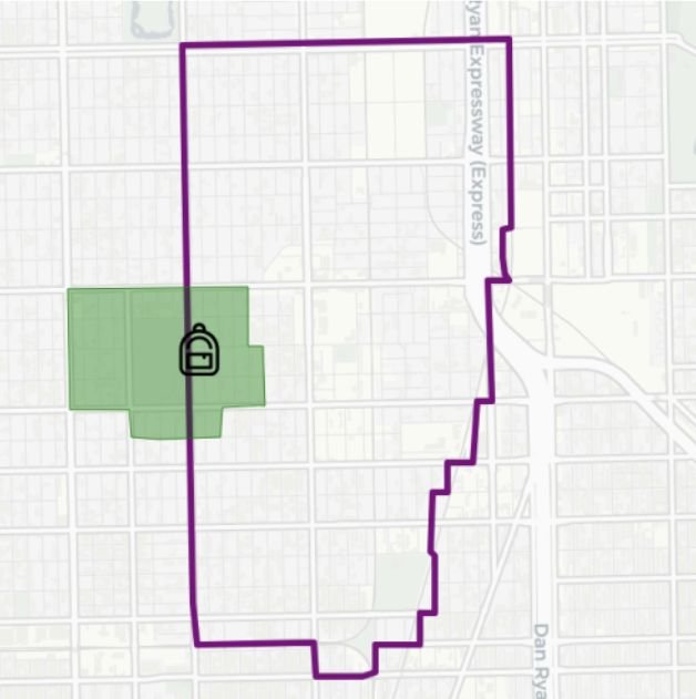
A map showing the overlap between the Englewood community area and the Bass Elementary School attendance boundaries.
school weight = student enrollment × attendance boundary overlap
community area weighted average = (sum of measure × weight for each school) / sum of weight for each school
This resource explains weighted averages and their mathematical formula in more detail.
If measures are reported for both semesters of the school year, we create an annual value by taking the average of both weighted semester values.
annual value = (semester 1 weighted value + semester 2 weighted value) / 2
A list of all schools considered in the calculation process, their attendance boundary overlap, their enrollment, and the weighted number of students allocated to the community is available in the Education data notes on each profile page.
3. A few indicators: already aggregated to community areas
A few sources skip this process because they already publish data aggregated to the community area level. We don't calculate anything for these indicators; the number shown is the same one that the source publishes.
The tradeoff is coverage. Since we never break these indicators down to the tract level, our common building block for translating between geographies, we can't reassemble them for a ward or school board district. So these indicators appear in community area profiles only.
Statistical limitations: understanding precision
Every estimate here uses the same rigorous methods that government agencies and researchers use to track population trends nationwide. Each one comes with information about how much the actual value may vary from the estimate. This is called margin of error, and it lets you judge whether and how precisely you can rely on the estimate in your particular work.
Margin of error
When their source provides it, estimates on our site are presented with their respective margin of error. This number tells you how much the actual value may vary from the estimate, within a 90% confidence interval.
If Albany Park had a 10% unemployment rate in 2018, with a 2% margin of error, then that means that we are 90% confident the actual unemployment rate for Albany Park is between 8% and 12%, or between estimate - margin of error and estimate + margin of error.
Here is a resource directly from the U.S. Census Bureau that explains margin of error in further detail.
Standard error
There is a related term, standard error, that can be derived from the margin of error (and vice versa). We use standard error under the hood to aggregate margins of error from one geographic level to another.
The coefficient of variation
In order to assess if an estimate’s margin of error rendered it reliable or unreliable, we used a metric called the coefficient of variation, which is equal to: the estimate’s standard error / estimate
There are no standard tiers for whether a CV is reliable—the level of acceptable (im)precision depends on your work. We offer the tiers outlined by Esri in their methodology for working with ACS data as a general guideline.
- Estimates with a CV of less than 0.12 is considered reasonably reliable and can be used as presented, e.g., 7.64.
- Estimates with a CV between 0.12 and 0.4 are considered reliable but imprecise and should be used approximately, e.g., about 7.
- Estimates with a CV of 0.4 or higher are imprecise and should be used as range equal to the approximate value ± the margin of error, i.e., between 5 and 9.
Note that estimates with a value of zero are unassessed, since division by 0 is arithmetically undefined.
If using values with relatively high margins of error, here are a few tips:
- Present the flagged estimate as “around this much,” not a precise value.
- Avoid reading into year-over-year changes, especially if values fall within the same error range.
- Where precision matters, consider using the citywide or community area value, rather than a subgroup estimate with a larger margin of error.
You can find the specific formulas we used to aggregate margins of error across geographic levels for sums, proportions, or medians here from the Census.
Additional sources we consulted to aggregate margins of error for median household income are this census-data-aggregator package from the LA Times, and this blog from Esri.
Survey data
Sampling. Many indicators come from the American Community Survey (ACS) 5-Year estimates. The ACS produces estimates based on surveys of randomly selected representative samples of the population. The bigger the sample population, the more likely the representative sample matches the whole population, the smaller the estimate’s margin of error will be. In other words, the margin of error tends to be smaller as the population size grows, i.e., subgroup estimates are the least precise, while citywide estimates are the most precise.
Smoothing. To produce more precise estimates, the Census Bureau combines five years of survey responses into one 5-year estimate. The number labeled "2022" reflects responses gathered from 2018 through 2022. This gives a stable read on long-term conditions, best used for tracking gradual trends rather than isolating a single year. One tradeoff is that sudden shifts appear gradually across the data instead of all at once.
For trend analysis, the Census recommends comparing year ranges that do not overlap, e.g., 2014 (covering 2010-2014), 2019 (covering 2015-2019), and 2024 (covering 2020-2024).
They also note that survey response rates were much lower in 2020 than any other year, something to keep in mind when comparing estimates for 2020 with estimates from other years.
The Census explains what their multiyear estimates mean in more detail here. They also offer guidance for comparing estimates across different data release years here.
Population assumptions
Our calculations rely on simplifying assumptions, standard in this kind of analysis. Tract weighting assumes a tract's population is spread evenly across its area: that 63% of a tract's land counts as 63% of its population. This is called assumed uniform distribution (of population). We also assume uniform population distribution of students across a CPS attendance boundary.
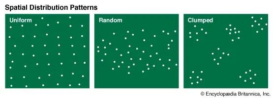
Examples of spatial distribution patterns: uniform, random, and clumped